        The Kennedy Thorndike Experiment: Doug Marett 2012 YouTube
video associated with
this article is here Introduction
The
Kennedy-Thorndike experiment was an experimental test of the
Lorentz-Einstein transformations. They considered the mathematical
treatment originally applied to the Michelson-Morley experiment to see
if there was a way to design an experiment to discriminate between
Lorentz ether theory and special relativity.
They
predicted that a Michelson interferometer exposed to different
velocities would experience a phase shift at the detector which was
proportional to the velocity, unless the frequency of the light depends
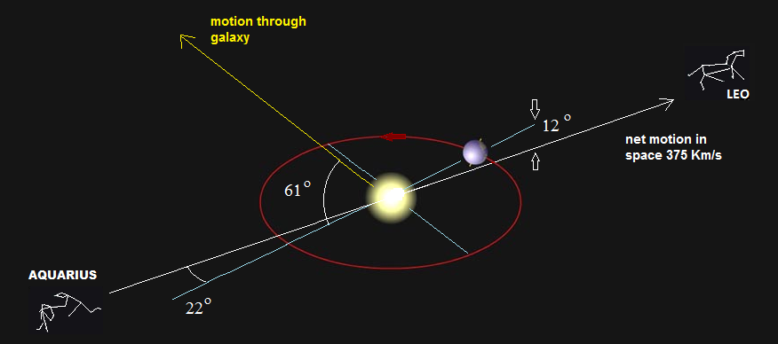
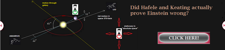
upon velocity in the way required by relativity. Consider the earth’s
absolute motion with respect to the Cosmic Microwave Background
Radiation (CMBr). We appear to moving at around 375 km/s towards the
constellation Leo. If we have a Michelson interferometer flat on the
surface of the earth pointing west, once a day the constellation Leo
will cross the western horizon, so the interferometer will be directly
aligned with our velocity through space. However, if we were to wait 6
hours after that moment, the interferometer would then be pointing
perpendicular to our motion. Although Kennedy and Thorndike were
unaware of the direction of our true net motion through space, they
hypothesized that as the interferometer moved in and out of the plane
of motion, whatever it is, a fringe shift should occur between the two
returning light beams from the arms, since they would be affected by
the relative motion in different ways depending on our orientation with
respect to space. Further, this fringe shift would be amplified if the
arms of the interferometer were different lengths.
The experiment relied on the
following assumptions: 1)
There
exists at least one coordinate system in which Huygen’s principle is
valid and the velocity of light is the same in all directions. For
Lorentz’s ether theory, this is any system at rest in the ether; for
relativity, this is all uniformly moving systems. 2)
That
some form of Lorentz contraction occurs in the direction of motion,
proportional to [1-v^2/c^2] ½ The
authors put forward as their primary goal to test the validity of the
time dilation effect in the moving frame of the interferometer – as
they state, “the theory has needed confirmation, particularly in its
most revolutionary aspect; i.e., its denial of a significance for
absolute time.” It was therefore an underlying premise of the
experiment that a null result should only occur if time dilation
happens on the moving interferometer as predicted by the theory of
relativity. Diagram of the Experiment: The interferometer used in the experiment is shown below.
The
interferometer arms were in a vacuum chamber and the interference
fringes were monitored using photographic plates mounted on a window to
the chamber. The arms were short (around 61 mm and 220 mm) and placed
at an angle of 56 degrees to one another. The device was not rotated -
the rotation of the Earth diurnally served as the primary means of
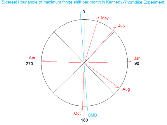
pointing in the arms in different directions in space. The experimental results: Diurnal Effects: Although the cardinal directions of the apparatus are not cited, along with a lot of other relevant details, the average maximum daily fringe shift per month was provided with the angle it points in sidereal time. This is only a two dimensional slice of the Azimuth angle, so the anisotropy could be anywhere between 0 and maximum depending on the Alt angle formed to the actual Alt direction of the CMBr. However, only the data from October is close to the Azimuth angle of the CMBr.
Kennedy
and Thorndike do a simple vector addition of the monthly anisotropies
to find the yearly average (based on their weighed values). This gives
a value of 0.06 thousands of a fringe shift (direction not given) which
corresponds to 24km/s. The seemingly random distribution of
anisotropies suggests that no clear direction was found, and that this
result is likely due to noise. Long Period
Effects: The
long period variations were on the order of 15km/s and were 123 degrees
away from the average for the daily variations. Where added
vectorially, this gave about 10km/s. This value is chosen as the value
of the null result, on the level of the M&M experiment. Simulation of the Kennedy-Thorndike
Experiment: In
order to show more clearly the predictions and expected results from
the Kennedy Thorndike experiment, an Excel simulation of it is provided
here
using Lorentz ether theory (LET). As will be shown shortly, Lorentz’s
exact theorem of 1904, which Kennedy and Thorndike did not take into
account, actually predicts the same outcome as Einstein’s special
theory of relativity (SR). Both use the Lorentz transformations, so
both predict an identical, null result. We make the following basic
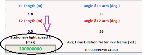
assumptions: 1) The speed of light is constant in the stationary frame – for LET this is a system at rest with respect to the ether. This input value is shown in the simulation below as 3 e 8 m/s.
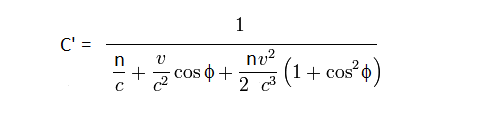
2) The one way speed of light in the moving frame can be calculated using an algebraic equation that includes the angle of orientation to the motion and the refractive index of the medium. We chose in this case to use an equation from Lorentz’s 1921 paper on the Michelson Morley experiment. I have modified this equation slightly to fully compensate for the effect of refractive index at second order, the final form of the equation is shown below:
n = Refractive index, c = speed of light in stationary frame, v is velocity of interferometer, and f is the angle between the arm and the direction of motion.
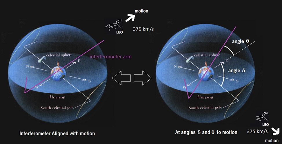
3) When calculating the final angle f which figures in both the velocity equation and in the Lorentz contraction applied, it is necessary to take into consideration the ultimate position of the arm vertically as well as horizontally from the direction of motion. To show this more clearly, a diagram is provided below which shows the Kennedy-Thorndike interferometer arms (in purple) superimposed on the earth in space. The movement of Leo is shown in two arbitrary positions, one aligned with the long arm, and the other nearly perpendicular, to highlight the horizontal and vertical angles that need to be calculated to arrive at the final velocity vector with respect to our motion through space:
In our simulation, we use the angle d and angle q to arrive at a final angle value f that can be applied directly into
our equation. The equation used for determining the value is: f = 90 – (90- q) * cos(d)
4) The time for light to traverse a given arm is calculated by taking the length of the arm, multiplying by the directionally dependent Lorentz contraction, and dividing by the one way speed of light. The directionally dependent Lorentz contraction is calculated as follows for each arm:
aLC = (1-v*cos(q)*cos(q)/c2)1/2
All forward and reverse paths for a given beam to reach the detector are added together. The sum is then multiplied by the time dilation factor a to determine the total local elapsed time for a given wave front to go from the source to the detector.
( Lforward * aLC/C’ + Lreverse * aLC/C’ ) * at = t’ sum in local time
[2L/( Lforward * aLC/C’ + Lreverse * aLC/C’ )] / at = C’ average in local time
Where L = path length in forward or reverse direction
The average speed of light for the entire trip is also shown below this value. In general, if time dilation and Lorentz contraction are applied, this value is always identical to the speed of light in the stationary frame ( C ) to a good approximation. 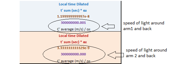
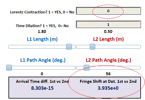
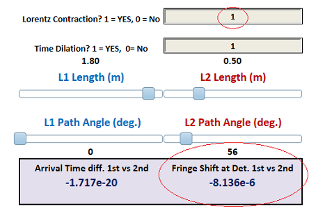
The simulator is set up with same angle of 56 degrees for the Kennedy-Thorndike interferometer arms, with the pre-loaded conditions having arms about 8x larger so they are more visible on the graph provided. In order to simulate a fringe shift, the Lorentz contraction part of the calculation can be disabled by setting the box [Lorentz contraction 1= Yes, 0 = No] to 0. When this is done, then a large fringe shift in the lower right hand box should appear. With the pre-loaded velocity of 375Km/s and with the second orientation at 80 degrees, the fringe shift should be around 3.9.
However, when the Lorentz contraction is applied [Lorentz contraction 1= Yes, 0 = No] = 1 then the fringe shift should then drop by around 6 orders of magnitude to around 8 e -6 fringes, as shown below:
The simulator is designed so that the arm lengths, the angles between the arms, and the velocities experienced by the interferometer, can all be adjusted, to show that none of these adjustments make any difference in the null result. However, if [Time dilation] = 0 is set, the average velocity for the speed of light, C’ will become different when the beams meet at the detector (but the fringe shift remains low). This difference is exactly proportional to the frequency shift on the moving source. If this box is reset to 1, then the speed of light for each returning beam C’ becomes = 3e8 m/s again.
The
Kennedy-Thorndike experiment demonstrates that Lorentz’s original
proposition of the Lorentz contraction and time dilation are
experimentally testable hypotheses – using the formulas above,
predictions can be made as to the anticipated results, and they can be
compared to the results of real experiments to see if the hypothesis is
proven true or false. . Lorentz did not anticipate the
Kennedy-Thorndike experiment, and as can be seen from the simulation,
the only way that we arrive at the correct experimental result is if
both of these effects are true. So this experiment stands as a proper
test of LET. As will be shown in another
simulation,
Lorentz’s theorem also predicts the Sagnac effect, a positive outcome
not anticipated by Lorentz since the Sagnac experiment was first
performed in 1913. Another interesting feature is that the predicted
result is unaffected by a change in the refractive index of the arms.
This feature shows that LET is entirely consistent with the
experimental results of the Shamir and Fox experiment of 1969. A
separate Shamir and Fox simulator is available here. To
quote M. Ruderfer:
“The
null result obtained by Shamir and Fox for the Michelson-Morley
experiment performed in a solid transparent medium does not distinguish
between special relativity and stationary (Lorentz) ether theories, as
claimed. Ives has shown that in the stationary ether theory the
measured one-way velocity of light in a translating refracting medium
is independent of the velocity of the medium through the ether.” What
does it mean to say that time dilation is occurring in the
interferometer?
What
is implied is that the frequency of the light moving in the
interferometer differs from the frequency it would have in its
stationary state (Jannsen
p.53).
One would also expect that the measured rate of time (local time for
Lorentz) will differ from that in the stationary frame. Lorentz saw
this as a mathematical stipulation device, whereas Einstein saw this a
change in the rate of real time. So
what does it actually mean? 1)
The
frequency of the light in the interferometer arms changes based on f/g or f * a - this
is orientation independent, since regardless of the direction the
source is pointing, the frequency shift (apparent time dilation) is
always proportional to a. 2)
The
one way wavelength of the light and one way speed of light change at
first order in an orientation dependent way. Using C = fl, if the one way velocity of light
decreases, the wavelength decreases. The
explanation using Lorentz ether theory evolves a little differently
than one using SR, since in the former case we are starting from a
stationary frame with Newtonian time, and working forward to a moving
frame using local time that is dilated with respect to the former. This
local time would be equivalent to “proper time” in SR. I use the factor
a
in the former case to express the time dilation, although the result is
the same as in SR, namely that the moving frame is the one with the
longer period for one second. Conclusions
It
had previously been argued by Popper that Lorentz’s concept of the
Lorentz-Fitzgerald contraction hypothesis was an unsatisfactory
auxiliary hypothesis that had no falsifiable consequences. A. Grunbaum
later argued that based on the Kennedy Thorndike experiment, the
Lorentz contraction hypothesis was in fact testable, but somehow came
to the conclusion that this experiment proved the hypothesis false.
However, Grunbaum relies on the older mathematical arguments prior to
Lorentz’s exact theorem of corresponding states (1899,1904) which
generated both the Lorentz transformation and took into account first
and second order effects experienced by interferometers used to try to
detect our motion through space. This more developed theory of Lorentz
has been defended by several authors, including Mansouri and Sexl,
Tyapkin, and Ruderfer, as remaining consistent with the predictions of
SR in virtually every optical experiment. Using this more advanced
treatment, it can be shown that the Kennedy Thorndike experimental
result is entirely in keeping with the predictions of LET - the Lorentz
contraction is required for the null result, and the effect of time
dilation on the moving source is required to maintain the two-way
average velocity of light as equal to C. This
is true regardless of whether time dilation is considered real or
apparent. References: 1)
Kennedy,
Roy, Thorndike, Edward, (1932) Physical Review Vol. 42, p. 400-418. 2)
Grunbaum,
A. The
Falsifiability of the Lorentz-Fitzgerald Contraction Hypothesis. The British Journal for the
Philosophy of Science, Vol.10, No.37. (May,1959), pp. 48-50. 3)
Mansouri,
R.,Sexl, R., A
Test of Special Relativity: III. Second Order Tests. Gen.
Rel. Grav. Vol. 8, No. 10 (1977) p. 809.814. 4)
Tyapkin.,
A.A.., (1973) "On the Impossibility of the First-Order Relativity
Test." Lettere Al Nuovo Cimento Vol. 7,
No. 15, 760-764. 5)
Ruderfer,
M. Comment On: A New Experimental Test of Special Relativity. Lettere
Al Nuovo Cimento Vol. 3, No. 21, 658-662. 6)
Shamir,
J., Fox, R., (1969) Il Nuovo Cimento Vol. 62B, No. 2 p.
258-264. |